dgrid3d

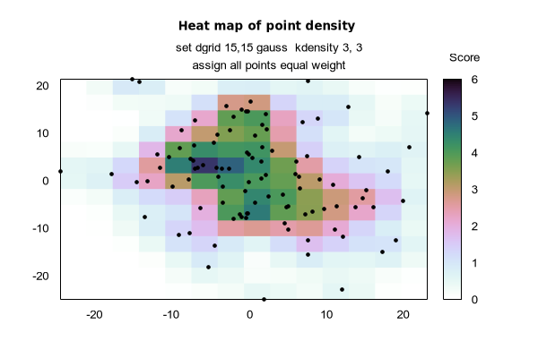
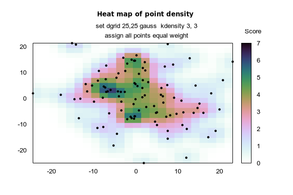
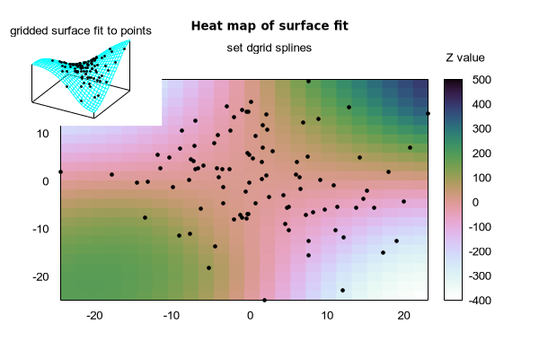
The set dgrid3d command enables and sets parameters for mapping non-grid data onto a grid. See splot grid_data for details about the grid data structure. Aside from its use in fitting 3D surfaces, this process can also be used to generate 2D heatmaps, where the 'z' value of each point contributes to a local weighted value.

Syntax:

      set dgrid3d {<rows>} {,{<cols>}} splines
      set dgrid3d {<rows>} {,{<cols>}} qnorm {<norm>}
      set dgrid3d {<rows>} {,{<cols>}} {gauss | cauchy | exp | box | hann}
                      {kdensity} {<dx>} {,<dy>}
      unset dgrid3d
      show dgrid3d

By default dgrid3d is disabled. When enabled, 3D data points read from a file are treated as a scattered data set used to fit a gridded surface. The grid dimensions are derived from the bounding box of the scattered data subdivided by the row/col_size parameters from the set dgrid3d statement. The grid is equally spaced in x (rows) and in y (columns); the z values are computed as weighted averages or spline interpolations of the scattered points' z values. In other words, a regularly spaced grid is created and then a smooth approximation to the raw data is evaluated for each grid point. This surface is then plotted in place of the raw data.

While dgrid3d mode is enabled, if you want to plot individual points or lines without using them to create a gridded surface you must append the keyword nogrid to the corresponding splot command.

The number of columns defaults to the number of rows, which defaults to 10.

Several algorithms are available to calculate the approximation from the raw data. Some of these algorithms can take additional parameters. These interpolations are such that the closer the data point is to a grid point, the more effect it has on that grid point.

The splines algorithm calculates an interpolation based on thin plate splines. It does not take additional parameters.

The qnorm algorithm calculates a weighted average of the input data at each grid point. Each data point is weighted by the inverse of its distance from the grid point raised to some power. The power is specified as an optional integer parameter that defaults to 1. This algorithm is the default.

Finally, several smoothing kernels are available to calculate weighted averages: z = Sum_i w(d_i) * z_i / Sum_i w(d_i), where z_i is the value of the i-th data point and d_i is the distance between the current grid point and the location of the i-th data point. All kernels assign higher weights to data points that are close to the current grid point and lower weights to data points further away.

The following kernels are available:

      gauss :     w(d) = exp(-d*d)
      cauchy :    w(d) = 1/(1 + d*d)
      exp :       w(d) = exp(-d)
      box :       w(d) = 1                     if d<1
                       = 0                     otherwise
      hann :      w(d) = 0.5*(1+cos(pi*d))     if d<1
                  w(d) = 0                     otherwise

When using one of these five smoothing kernels, up to two additional numerical parameters can be specified: dx and dy. These are used to rescale the coordinate differences when calculating the distance: d_i = sqrt( ((x-x_i)/dx)**2 + ((y-y_i)/dy)**2 ), where x,y are the coordinates of the current grid point and x_i,y_i are the coordinates of the i-th data point. The value of dy defaults to the value of dx, which defaults to 1. The parameters dx and dy make it possible to control the radius over which data points contribute to a grid point IN THE UNITS OF THE DATA ITSELF.

The optional keyword kdensity, which must come after the name of the kernel, but before the optional scale parameters, modifies the algorithm so that the values calculated for the grid points are not divided by the sum of the weights ( z = Sum_i w(d_i) * z_i ). If all z_i are constant, this effectively plots a bivariate kernel density estimate: a kernel function (one of the five defined above) is placed at each data point, the sum of these kernels is evaluated at every grid point, and this smooth surface is plotted instead of the original data. This is similar in principle to what the smooth kdensity option does to 1D datasets. See kdensity2d.dem and heatmap_points.dem for usage example.

The dgrid3d option is a simple scheme which replaces scattered data with weighted averages on a regular grid. More sophisticated approaches to this problem exist and should be used to preprocess the data outside gnuplot if this simple solution is found inadequate.

See also the online demos for dgrid3d scatter and heatmap_points