
# # $Id: fit.dem,v 1.8 2009/10/31 05:24:18 sfeam Exp $ # print "Some examples how data fitting using nonlinear least squares fit" print "can be done." print ""Click here for minimal script to generate this plot
|
| # # $Id: fit.dem,v 1.8 2009/10/31 05:24:18 sfeam Exp $ # print "Some examples how data fitting using nonlinear least squares fit" print "can be done." print "" |
|
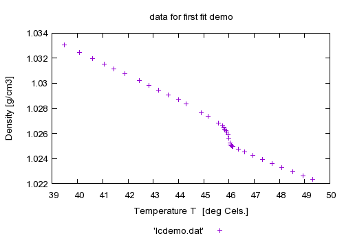
set title 'data for first fit demo' set xlabel "Temperature T [deg Cels.]" set ylabel "Density [g/cm3]" set key below plot 'lcdemo.dat' print "now fitting a straight line to the data :-)" print "only as a demo without physical meaning" load 'line.fnc' y0 = 0.0 m = 0.0 print "fit function and initial parameters are as follows:" print GPFUN_l show variables y0 show variables m #show variables |
|
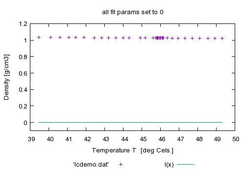
set title 'all fit params set to 0' plot [*:*][-.1:1.2] 'lcdemo.dat', l(x) print "fit command will be: fit l(x) 'lcdemo.dat' via y0, m" |

|
fit l(x) 'lcdemo.dat' via y0, m |
|
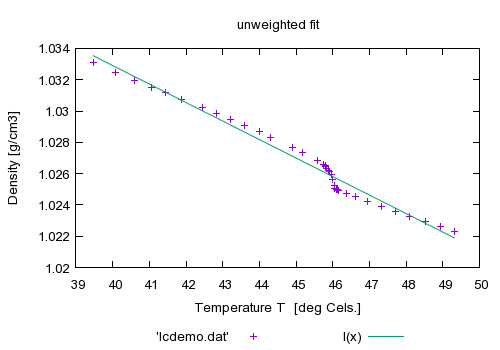
set title 'unweighted fit' plot 'lcdemo.dat', l(x) print "" print "now fit with weights from column 3 which favor low temperatures" print "command will be: fit l(x) 'lcdemo.dat' using 1:2:3 via y0, m" |

|
fit l(x) 'lcdemo.dat' using 1:2:3 via y0, m |
|
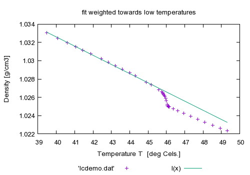
set title 'fit weighted towards low temperatures' plot 'lcdemo.dat', l(x) print "" print "now fit with weights from column 4 instead" print "command will be: fit l(x) 'lcdemo.dat' using 1:2:4 via y0, m" |

|
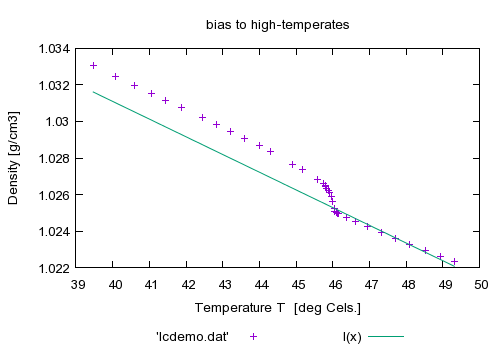
fit l(x) 'lcdemo.dat' using 1:2:4 via y0, m |
|
set title 'bias to high-temperates' plot 'lcdemo.dat', l(x) |
|
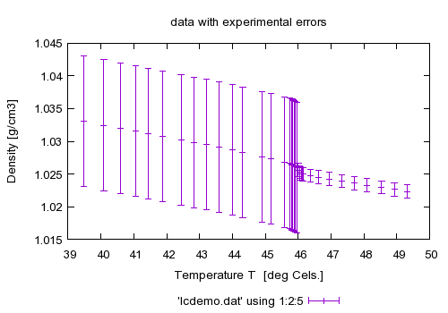
set title 'data with experimental errors' plot 'lcdemo.dat' using 1:2:5 with errorbars print "" print "now use these real single-measurement errors from column 5 to reach " print "such a result (look at the file lcdemo.dat and compare the columns to " print "see the difference)" print "command will be: fit l(x) 'lcdemo.dat' using 1:2:5 via y0, m" |

|
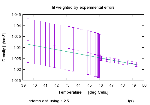
fit l(x) 'lcdemo.dat' using 1:2:5 via y0, m |
|
set title 'fit weighted by experimental errors' plot 'lcdemo.dat' using 1:2:5 with errorbars, l(x) |
|
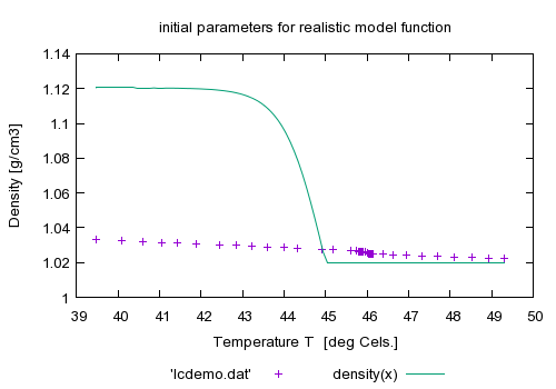
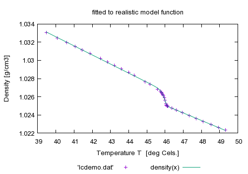
load 'density.fnc' set title 'initial parameters for realistic model function' plot 'lcdemo.dat', density(x) print "" print "It's time now to try a more realistic model function:" print GPFUN_density print GPFUN_curve print GPFUN_lowlin print GPFUN_high #show functions print "density(x) is a function which shall fit the whole temperature" print "range using a ?: expression. It contains 6 model parameters which" print "will all be varied. Now take the start parameters out of the" print "file 'start.par' and plot the function." print "command will be: fit density(x) 'lcdemo.dat' via 'start.par'" load 'start.par' |

|
fit density(x) 'lcdemo.dat' via 'start.par' |
|
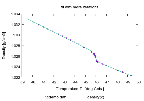
set title 'fitted to realistic model function' plot 'lcdemo.dat', density(x) print "" print "looks already rather nice? We will do now the following: set" print "the epsilon limit higher so that we need more iteration steps" print "to convergence. During fitting please hit ctrl-C. You will be asked" print "Stop, Continue, Execute: Try everything. You may define a script" print "using the FIT_SCRIPT environment variable. An example would be" print "'FIT_SCRIPT=plot nonsense.dat'. Normally you don't need to set" print "FIT_SCRIPT since it defaults to 'replot'. Please note that FIT_SCRIPT" print "cannot be set from inside gnuplot." print "" print "command will be: fit density(x) 'lcdemo.dat' via 'start.par'" |

|
FIT_LIMIT = 1e-10 fit density(x) 'lcdemo.dat' via 'start.par' |
|
set title 'fit with more iterations' plot 'lcdemo.dat', density(x) |

|
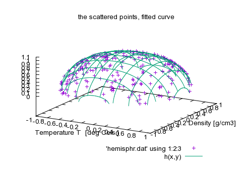
FIT_LIMIT = 1e-5 print "\nNow a brief demonstration of 3d fitting." print "hemisphr.dat contains random points on a hemisphere of" print "radius 1, but we let fit figure this out for us." print "It takes many iterations, so we limit FIT_MAXITER to 50." #HBB: made this a lot harder: also fit the center of the sphere #h(x,y) = sqrt(r*r - (x-x0)**2 - (y-y0)**2) + z0 #HBB 970522: distort the function, so it won't fit exactly: h(x,y) = sqrt(r*r - (abs(x-x0))**2.2 - (abs(y-y0))**1.8) + z0 x0 = 0.1 y0 = 0.2 z0 = 0.3 r=0.5 FIT_MAXITER=50 set title 'the scattered points, and the initial parameter' splot 'hemisphr.dat' using 1:2:3, h(x,y) print "fit function will be: " . GPFUN_h print "we *must* provide 4 columns for a 3d fit. We fake errors=1" print "command will be: fit h(x,y) 'hemisphr.dat' using 1:2:3:(1) via r, x0,y0,z0" |
|
# we *must* provide 4 columns for a 3d fit. We fake errors=1 fit h(x,y) 'hemisphr.dat' using 1:2:3:(1) via r, x0, y0, z0 set title 'the scattered points, fitted curve' splot 'hemisphr.dat' using 1:2:3, h(x,y) print "\n\nNotice, however, that this would converge much faster when" print "fitted in a more appropriate co-ordinate system:" print "fit r 'hemisphr.dat' using 0:($1*$1+$2*$2+$3*$3) via r" print "where we are fitting f(x)=r to the radii calculated as the data" print "is read from the file. No x value is required in this case." |
|
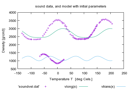
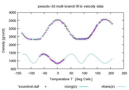
FIT_MAXITER=0 # no limit : we cannot delete the variable once set print "\n\nNow an example how to fit multi-branch functions\n" print "The model consists of two branches, the first describing longitudinal" print "sound velocity as function of propagation direction (upper data, from " print "dataset 1), the second describing transverse sound velocity (lower " print "data, from dataset 0).\n" print "The model uses these data in order to fit elastic stiffnesses" print "which occur differently in both branches." load 'hexa.fnc' load 'sound.par' set title 'sound data, and model with initial parameters' plot 'soundvel.dat', vlong(x), vtrans(x) print "" print "fit function will be: " . GPFUN_f print GPFUN_vlong print GPFUN_vtrans print "y will be the index of the dataset" print "command will be: fit f(x,y) 'soundvel.dat' using 1:-2:2:(1) via 'sound.par'" |

|
# Must provide an error estimate for a 3d fit. Use constant 1 fit f(x,y) 'soundvel.dat' using 1:-2:2:(1) via 'sound.par' #create soundfit.par, reading from sound.par and updating values update 'sound.par' 'soundfit.par' print "" |
|
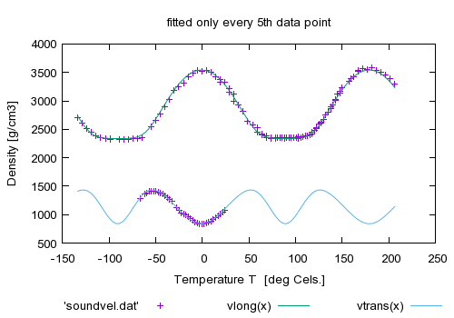
set title 'pseudo-3d multi-branch fit to velocity data' plot 'soundvel.dat', vlong(x), vtrans(x) print "Look at the file 'hexa.fnc' to see how the branches are realized" print "using the data index as a pseudo-3d fit" print "" print "Next we only use every fifth data point for fitting by using the" print "'every' keyword. Look at the fitting-speed increase and at" print "fitting result." print "command will be: fit f(x,y) 'soundvel.dat' every 5 using 1:-2:2:(1) via 'sound.par'" |
|
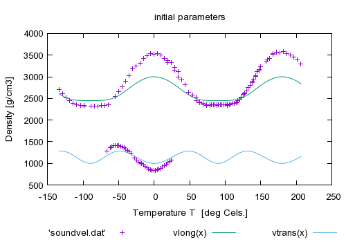
load 'sound.par' fit f(x,y) 'soundvel.dat' every 5 using 1:-2:2:(1) via 'sound.par' set title 'fitted only every 5th data point' plot 'soundvel.dat', vlong(x), vtrans(x) print "When you compare the results (see 'fit.log') you remark that" print "the uncertainties in the fitted constants have become larger," print "the quality of the plot is only slightly affected." print "" print "By marking some parameters as '# FIXED' in the parameter file" print "you fit only the others (c44 and c13 fixed here)." print "" |
|
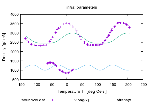
load 'sound2.par' set title 'initial parameters' plot 'soundvel.dat', vlong(x), vtrans(x) fit f(x,y) 'soundvel.dat' using 1:-2:2:(1) via 'sound2.par' set title 'fit with c44 and c13 fixed' plot 'soundvel.dat', vlong(x), vtrans(x) print "This has the same effect as specifying only the real free" print "parameters by the 'via' syntax." print "" print "fit f(x) 'soundvel.dat' via c33, c11, phi0" print "" |
|
load 'sound.par' set title 'initial parameters' plot 'soundvel.dat', vlong(x), vtrans(x) fit f(x,y) 'soundvel.dat' using 1:-2:2:(1) via c33, c11, phi0 set title 'fit via c33,c11,phi0' plot 'soundvel.dat', vlong(x), vtrans(x) print "Here comes an example of a very complex function..." print "" |
|
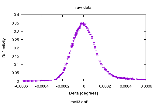
set xlabel "Delta [degrees]" set ylabel "Reflectivity" set title 'raw data' #HBB 970522: here and below, use the error column present in moli3.dat: plot 'moli3.dat' w e print "now fitting the model function to the data" load 'reflect.fnc' #HBB 970522: Changed initial values to something sensible, i.e. # something an experienced user of fit would actually use. # FIT_LIMIT is also raised, to ensure a better fit. eta = 1.2e-4 tc = 1.8e-3 FIT_LIMIT=1e-10 #show variables #show functions |
|
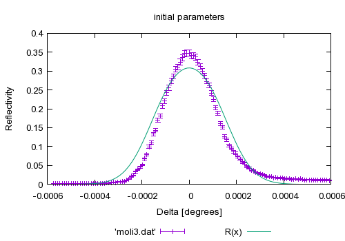
set title 'initial parameters' plot 'moli3.dat' w e, R(x) print "fit function is: " . GPFUN_R print GPFUN_a print GPFUN_W print "command will be: fit R(x) 'moli3.dat' u 1:2:3 via eta, tc" |

|
fit R(x) 'moli3.dat' u 1:2:3 via eta, tc |
|
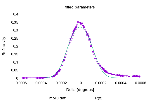
set title 'fitted parameters' replot #HBB 970522: added comment on result of last fit. print "Looking at the plot of the resulting fit curve, you can see" print "that this function doesn't really fit this set of data points." print "This would normally be a reason to check for measurement problems" print "not yet accounted for, and maybe even re-think the theoretic" print "prediction in use." print "" |
|
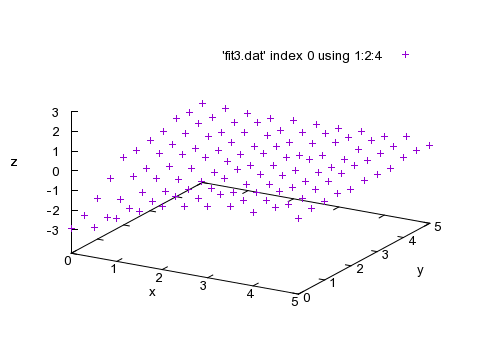
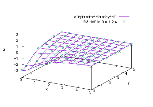
set xlabel 'x' set ylabel 'y' set zlabel 'z' set ticslevel .2 set zrange [-3:3] splot 'fit3.dat' index 0 using 1:2:4 print '' print 'Next we show a fit with three independent variables. The file' print 'fit3.dat has four columns, with values of the three independent' print 'variable x, y, and t, and the resulting value z. The data' print 'lines are in four sections, with t being constant within each' print 'section. The sections are separated by two blank lines, so we' print 'can select sections with "index" modifiers. Here are the data in' print 'the first section, where t = -3.' print '' print 'We will fit the function a0/(1 + a1*x**2 + a2*y**2) to these' print 'data. Since at this point we have two independent variables,' print 'our "using" spec has four entries, representing x:y:z:s (where' print 's is the estimated error in the z value).' print "Command will be: " print " fit a0/(1+a1*x**2+a2*y**2) 'fit3.dat' index 0 using 1:2:4:(1) via a0,a1,a2" |

|
a0=1; a1=.1; a2=.1 fit a0/(1+a1*x**2+a2*y**2) 'fit3.dat' index 0 using 1:2:4:(1) via a0,a1,a2 |
|
splot a0/(1+a1*x**2+a2*y**2), 'fit3.dat' in 0 u 1:2:4 |
|
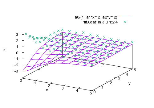
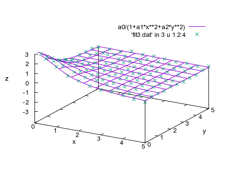
splot a0/(1+a1*x**2+a2*y**2), 'fit3.dat' in 3 u 1:2:4 print "" print "Here is the last set of data where t = 3." print "We fit the same function to this set." print "Command will be: " print " fit a0/(1+a1*x**2+a2*y**2) 'fit3.dat' in 3 u 1:2:4:(1) via a0,a1,a2" |

|
fit a0/(1+a1*x**2+a2*y**2) 'fit3.dat' in 3 u 1:2:4:(1) via a0,a1,a2 |
|
splot a0/(1+a1*x**2+a2*y**2), 'fit3.dat' in 3 u 1:2:4 |
|
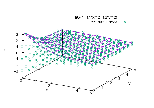
splot a0/(1+a1*x**2+a2*y**2), 'fit3.dat' u 1:2:4 print "" print "We also have data for several intermediate values of t. We" print "will fit the function f(x,y,t)=a0*t/(1+a1*x**2+a2*y**2) to all" print "the data. Since there are now three independent variables, we" print "need a using spec with five entries, representing x:y:t:z:s." print "Command will be: " print " fit f(x,y,t) 'fit3.dat' u 1:2:3:4:(1) via a0,a1,a2" |

|
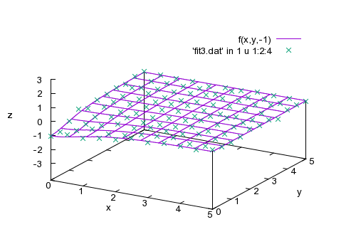
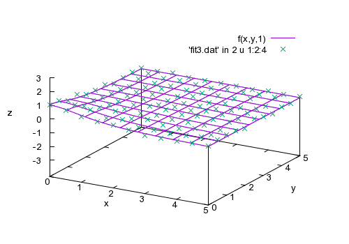
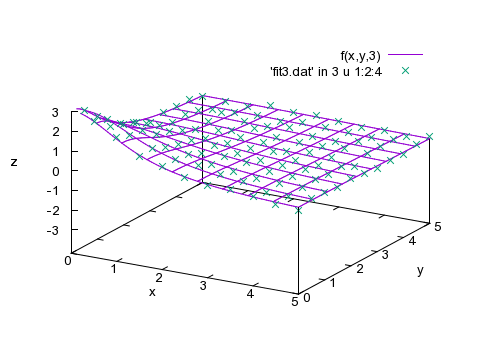
f(x,y,t)=a0*t/(1+a1*x**2+a2*y**2) fit f(x,y,t) 'fit3.dat' u 1:2:3:4:(1) via a0,a1,a2 print "We plot the data in each section with the corresponding" print "function values." |

|
splot f(x,y,-3), 'fit3.dat' in 0 u 1:2:4 |
|
splot f(x,y,-1), 'fit3.dat' in 1 u 1:2:4 |
|
splot f(x,y,1), 'fit3.dat' in 2 u 1:2:4 |
|
splot f(x,y,3), 'fit3.dat' in 3 u 1:2:4 |
|
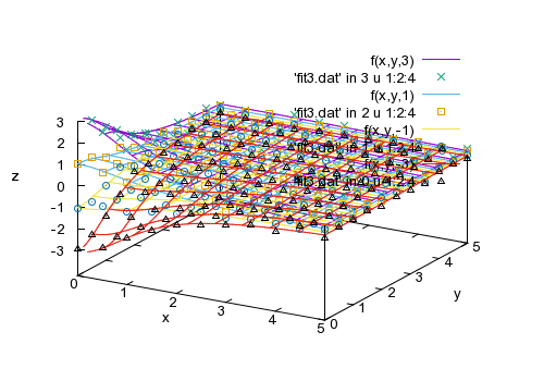
splot f(x,y,3), 'fit3.dat' in 3 u 1:2:4, \
f(x,y,1), 'fit3.dat' in 2 u 1:2:4, \
f(x,y,-1), 'fit3.dat' in 1 u 1:2:4, \
f(x,y,-3), 'fit3.dat' in 0 u 1:2:4
print 'Here are all the data together.'
print ''
print 'You can use ranges to rename variables and/or limit the data'
print 'included in the fit. The first range corresponds to the first'
print '"using" entry, etc. For example, we could have gotten the same'
print 'fit like this:'
print ' fit [lon=*:*][lat=*:*][time=*:*] \'
print ' a0*time/(1 + a1*lon**2 + a2*lat**2) \'
print ' "fit3.dat" u 1:2:3:4:(1) via a0,a1,a2'
print ''
print "You can have a look at all previous fit results by looking into"
print "the file 'fit.log' or whatever you defined the env-variable 'FIT_LOGFILE'."
print "Remember that this file will always be appended, so remove it"
print "from time to time!"
print ""
|

|
|