Back to demo index

gnuplot demo script: sectors.dem

autogenerated by webify.pl on Sun Sep 17 19:55:27 2023
gnuplot version gnuplot 6.0 patchlevel rc2
#########################################################
# Fig.5: parameters for specifying an annular sector
#########################################################
#

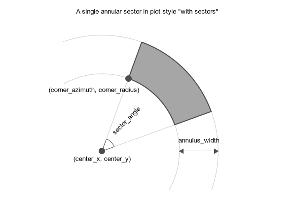
set title 'A single annular sector in plot style "with sectors"'

set polar
set angles degree
set theta top cw
set xrange [-3:10]
set yrange [-3:10]
set size ratio -1
unset border
unset raxis
unset tics
unset key

array data[1]

set arrow 1 from 6,0 to 9,0 
set arrow 1 heads size screen 0.015, 30, 90 filled front lw 1 lc rgb "gray30"

plot \
     data using (-30):(6):(300):(3) with sectors lc rgb "gray80" lw 1,\
     data using (20):(0):(50):(6)   with sectors lc rgb "gray80" lw 1,\
     data using (20):(6):(50):(3)   with sectors lc rgb "gray30" lw 2 fill solid 0.5 border,\
     data using (20):(0):(50):(1)   with sectors lc rgb "gray30" lw 1,\
     data using (20):(6)            with points pt 7 ps 2 lc rgb "gray30", \
     data using (0):(0)             with points pt 7 ps 2 lc rgb "gray30", \
     data using (0):(0):("(center_x, center_y)")     with labels offset 0,-1 noenhanced, \
     data using (0):(0):("sector_angle") with labels offset 7,4.2 noenhanced rotate by 45, \
     data using (90):(7.5):("annulus_width") with labels offset 0,1.5 noenhanced, \
     data using (20):(6):("(corner_azimuth, corner_radius)") with labels offset -10,-1.5 noenhanced


Click here for minimal script to generate this plot


#########################################################
# Fig.2: polar heatmap positioned in cartesian coordinate
#        system.  Note that the two halves of the plot
#        displaced by shifting the center to x = +/- 0.5.
#########################################################
#

set title "Polar heatmap composed of sectors\n"\
          ."positioned on a cartesian x/y plane"

rmax = 10
dr = 0.5
tmax = 180
dt = 10

f(t,r) = r*cos(t+20*r)**2

set angle degrees
set theta top cw
set xrange [-(rmax+2):(rmax+2)]
set yrange [-(rmax+2):(rmax+2)]
set size ratio -1
unset border
unset tics
unset key

set palette viridis
set colorbox user size 0.05, 0.5 origin 0.85,0.25
set cbtics

set table $data
set view map
splot sample [t=0:tmax-dt:dt] [r=0:rmax-dr:dr] "++" using (t):(r):(0)
unset table

plot $data using 1:2:(dt):(dr):(0.5):(0):(f($1+dt/2,$2+dr/2)) with sectors fc palette fill solid, \
     $data using (-$1):2:(-dt):(dr):(-0.5):(0):(f($1+dt/2,$2+dr/2)) with sectors fc palette fill solid


Click here for minimal script to generate this plot


############################################
# Yes/No survey results aggregated by groups
# Illustrates multiple sector plots in polar
# coordinate mode for the overall graph.
############################################
#

set label 1 at screen 0.1, 0.9
set label 1 "Multiple sector plots\npositioned on a polar graph"
set lmargin at screen 0.3

$data <<EOD
# Group Yes No
A 12 8 4
B 20 14 6
C 25 18 7
D 21 8 13 
E 10 2 8
EOD

stats $data using 2 nooutput
fac = 360.0/STATS_sum

set table $data2
plot r=0 $data using (sprintf("%s",strcol(1))):2:3:4:(r):(dr=$2*fac,r=r+dr,dr) with table
unset table

# print $data2

set polar
set angle degrees
set theta top cw

set xrange [-18:18]
set yrange [-18:18]
set size ratio -1

unset border
unset tics
unset raxis
unset key

set label 2 sprintf("TOTAL\n%d",STATS_sum) at 0,0 center offset 0,0.5

plot \
     $data2 using 5:(3):6:(4) with sectors fc rgb 'blue' lw 2 fill solid 0.2 border lc bgnd, \
     $data2 using 5:(7):6:(8) with sectors fc rgb 'blue' lw 2 fill solid 0.2 border lc bgnd, \
     $data2 using 5:(15):6:(3) with sectors fc rgb 'blue' lw 2 fill solid 0.2 border lc bgnd, \
     $data2 using ($5+$6/2):(16.5):(strcol(1)) with labels center font ",9", \
     $data2 using ($5+$6/2):(5):(sprintf("%.0f%%",100*$2/STATS_sum)) with labels center font ",9", \
     $data2 using ($5+$6/2):(11.1):(sprintf("%.0f%%",100*$3/$2)) with labels center font ",9", \
     $data2 using (0):(1.7):(361):(1.3):($5+$6/2):(11) with sectors fill solid 0.1 noborder fc bgnd, \
     $data2 using (0):(1.7):($3/$2*360):(1.3):($5+$6/2):(11) with sectors fill solid 0.4 noborder fc rgb "red"


Click here for minimal script to generate this plot


#########################################################
# Fig.3: pie (donut) chart
#########################################################
#

set title "Pie (donut) chart drawn with sectors"

$data <<EOD
1 100 0
2  70 1
3  60 0
4  50 0
5  40 1
6  30 0
7  10 0
EOD

stats $data using 2 nooutput
fac = 360.0/STATS_sum

set table $data2
plot r=0 $data using 1:2:3:(r):(dr=$2*fac,r=r+dr,dr) with table
unset table

set polar
set angles degree
set theta top cw
set xrange [-10:10]
set yrange [-10:10]
set size ratio -1
unset border 
unset raxis
unset tics
unset key

plot $data2 using 4:(4):5:(3):($0+1) with sectors lc variable lw 3 fill solid border lc bgnd, \
     $data2 using ($4+$5/2):(8+0.7*$3):(sprintf("%.1f",$2)) with labels


Click here for minimal script to generate this plot


set title "Pie (donut) chart some slices have radial shift"
plot $data2 using 4:(4+0.7*$3):5:(3):($0+1) with sectors lc variable lw 3 fill solid border lc bgnd, \
     $data2 using ($4+$5/2):(8+0.7*$3):(sprintf("%.1f",$2)) with labels


Click here for minimal script to generate this plot


set title "Pie (donut) chart some slices have offset origin"
plot $data2 using 4:(4):5:(3):($4+$5/2):(0.7*$3):($0+1) with sectors lc variable lw 3 fill solid border lc bgnd, \
     $data2 using ($4+$5/2):(8+0.7*$3):(sprintf("%.1f",$2)) with labels


Click here for minimal script to generate this plot


#########################################################
# Fig.4: dial charts
#########################################################
#

set title "Dial charts drawn with sectors"

$data <<EOD
-5  5 50 
 5  5 30 
-5 -5 80 
 5 -5 60 
EOD

set angle degrees
set theta left cw
set xrange [-10:10]
set yrange [-8:12]
unset border
unset tics
unset key

plot $data using (0):(1.5):(180):(2):1:2 with sectors units xx fc rgb 'gray' fill solid 1,\
     $data using (0):(1.5):($3/100*180):(2):1:2 with sectors units xx fc rgb 'blue' fill solid 1, \
     $data using 1:2:(strcol(3)) with labels offset 0,0.5


Click here for minimal script to generate this plot


#########################################################
# Fig.6: 'units' option
#########################################################
#

set angles degree
set theta top cw
set xrange [0:10]
set yrange [0:10]
unset key

array data[1]

set size 0.5, 0.5

set multiplot layout 2,2
set size noratio
plot \
     data using (20):(6):(50):(3)  with sectors lc rgb "gray30" lw 2 fill solid 0.5 border, \
     data using (20):(6):(360):(3) with sectors lc rgb "gray30" lw 1, \
     data using (0.5):(2):("noratio\nunits xy") with labels left

set size ratio -1
plot \
     data using (20):(6):(50):(3)  with sectors lc rgb "gray30" lw 2 fill solid 0.5 border, \
     data using (20):(6):(360):(3) with sectors lc rgb "gray30" lw 1, \
     data using (0.5):(2):("ratio -1\nunits xy") with labels left

set size noratio
plot \
     data using (20):(6):(50):(3)  with sectors units xx lc rgb "gray30" lw 2 fill solid 0.5 border, \
     data using (20):(6):(360):(3) with sectors units xx lc rgb "gray30" lw 1, \
     data using (0.5):(2):("noratio\nunits xx") with labels left

set size noratio
plot \
     data using (20):(6):(50):(3)  with sectors units yy lc rgb "gray30" lw 2 fill solid 0.5 border, \
     data using (20):(6):(360):(3) with sectors units yy lc rgb "gray30" lw 1, \
     data using (0.5):(2):("noratio\nunits yy") with labels left

unset multiplot


Click here for minimal script to generate this plot


#########################################################
# Fig.9 hue Circle (HSV model)
#########################################################
#


set polar
set angle degrees
set theta top cw

set size ratio -1
unset border
unset raxis
unset tics
unset key
unset colorbox

set xrange [-5:5]
set yrange [-5:5]
set cbrange [0:360]

da = 15

plot sample [t=0:360:da] \
     "+" using ($1-da/2.0):(2):(da):(2):(hsv2rgb($1/360,1,0.7)) with sectors \
                   fc rgb variable fill solid 1 border lc bgnd lw 2, \
     [t=0:360-da:da] "+" using ($1):(4.5):(sprintf("%i",$1)) with labels 


Click here for minimal script to generate this plot


#########################################################
# Fig.10 Wind rose (histgram on polar axis)
#########################################################
#


set title "Wind rose (polar coordinate histogram using sectors)"

$data <<EOD
# DIRECTION INDEX COUNT
N    1  10
NNE  2  15
NE   3  21
ENE  4  24
E    5  19
ESE  6  12
SE   7   8
SSE  8   4
S    9   2
SSW 10   4
SW  11   7
WSW 12  10
W   13  11
WNW 14   9
NW  15   5
NNW 16   7
EOD

stats $data using 2:3 nooutput

set polar
set angle degrees
set theta top cw

set xrange [-0.2:0.2]
set yrange [-0.2:0.2]
set size ratio -1

unset border
unset key
unset raxis
unset tics

array dummy[1]
plot $data using (22.5*($2-1-0.5)):(0.01):(22.5):($3/STATS_sum_y) with sectors \
              fc rgb "blue" fill solid 0.5 border lc bgnd, \
     for [k=0:15:5] dummy using (0):(0.01):(361):(k/100.0) with sectors lc rgb "gray30" lw 0.5 dt ".",\
     for [k=0:15:5] dummy using (0):(0.01+k/100.0):(sprintf("%d%%",k)) with labels offset 0,0.5 tc rgb "gray30"


Click here for minimal script to generate this plot


#########################################################
# Fig.11 Scanning overwraps
#########################################################
#


$data <<EOD
# x y angle_min angle_max range_min range_max
-3 0 -20 60 2 6
 3 0 -60 20 4 7
 -3 9 80 220 4 7
EOD

set angles degree
set theta top cw

set xrange [-8:8]
set yrange [-4:12]
set size ratio -1

unset border
unset key
unset tics

plot $data using 3:(0):($4-$3):5:1:2:($0+1) with sectors lc variable lw 1 dt 3, \
     $data using 1:2:($0+1) with points ps 3 pt 7 lc variable, \
     $data using 3:5:($4-$3):($6-$5):1:2:($0+1) with sectors lc variable lw 3 fill transparent solid 0.3


Click here for minimal script to generate this plot


#########################################################
# Fig.12 Pie charts (3 choices questionnaire)
#########################################################
#


$data <<EOD
# Question_NUM YES NO N/A
1 75 20 5
2 45 45 10
3 90 10 0
4 30 50 20
5 50 45 5
6 45 55 0
EOD

xpos(k) = 2*(int($0)%3)
ypos(k) = -2*(int($0)/3)

set angle degrees
set theta top cw

set xrange [-1:6]
set yrange [-3:1]
set size ratio -1

unset border
unset tics

set key noautotitle left Left reverse at graph 0.85, graph 0.80

plot $data using (0):(0.2):($2/100*360):(0.6):(xpos($0)):(ypos($0)) with sectors fill solid 0.5 noborder fc rgb "red" , \
     $data using ($2/100*360):(0.2):($4/100*360):(0.6):(xpos($0)):(ypos($0)) with sectors fill solid noborder fc rgb "gray", \
     $data using (0):(0.2):(-$3/100*360):(0.6):(xpos($0)):(ypos($0)) with sectors fill solid 0.5 noborder fc rgb "blue", \
     $data using (xpos($0)):(ypos($0)):(sprintf("Q.%d",$1)) with labels, \
     keyentry with boxes fill solid 0.5 noborder fc rgb "red" title "YES", \
     keyentry with boxes fill solid     noborder fc rgb "gray" title "N/A", \
     keyentry with boxes fill solid 0.5 noborder fc rgb "blue" title "NO"


Click here for minimal script to generate this plot


#########################################################
# Fig.13 Circular discrete gauge
#########################################################
#


set angles degrees
set theta top cw

set xrange [-8:8]
set yrange [-8:8]
set size ratio -1

unset border
unset tics
unset key

set style fill solid border lc rgb "gray"

plot sample [t=0:350:15] "+" using (t-5):(4):(10):(2) with sectors fc rgb "gray90" fill border lc black lw 2, \
            [t=0:220:15] "+" using (t-5):(4):(10):(2) with sectors fc rgb "orange" fill border lc black lw 2


Click here for minimal script to generate this plot


#########################################################
# Fig.14 Polar points with radial error
#########################################################
#


set title "Polar coordinate points with both radial and angular error\n" \
          . "represented by sectors"

set polar
set angles degree
set theta top cw
unset border 
unset raxis
unset tics
unset key

set xrange [-15:15]
set yrange [-15:15]
set size ratio -1

$data4 <<EOD
2 0.8
3 1.1
8 2.5
5 1.8
2 0.7
2 0.8
5 1.9
6 2.3
9 3.1
7 2.8
5 2.1
3 1.2
EOD

array dummy[1]

set style fill transparent solid 0.1 border
set grid polar lt 1 lc "gray60" lw 1.0 dt "-"
set rtics ("0" 3, "5" 8, "10" 13) left offset 0, 0.25

plot \
    dummy using (0):(0):(361):(3) with sectors fs solid bo lc "black" fc bgnd, \
    $data4 using (30*$0-15):(3+$1-$2/2.0):(30):($2) with sectors lt 6, \
    $data4 using (30*$0):(3):(0):($1) with vectors nohead lt 6 lw 1, \
    $data4 using (30*$0):(3+$1) with points pt 7 ps 1 lt 6


Click here for minimal script to generate this plot